Model atmosphere grids
Speedyfit is provided with 4 grids of model atmospheres. Below the range in effective temperature and surface gravity of all grids is shown. You can make these plots with the following python code:
import pylab as pl
from astropy.io import fits
from speedyfit.model import get_grid_file

grid = 'blackbody'

hdu = fits.open(get_grid_file(grid=grid, integrated=True))

teff = hdu[1].data['teff']
logg = hdu[1].data['logg']

pl.figure()
pl.plot(teff, logg, 'oC0')
pl.xlabel('Effective temperature [K]')
pl.ylabel('log(surface gravity) [cgs]')
pl.title('grid = ' + grid)
pl.tight_layout()

pl.show()
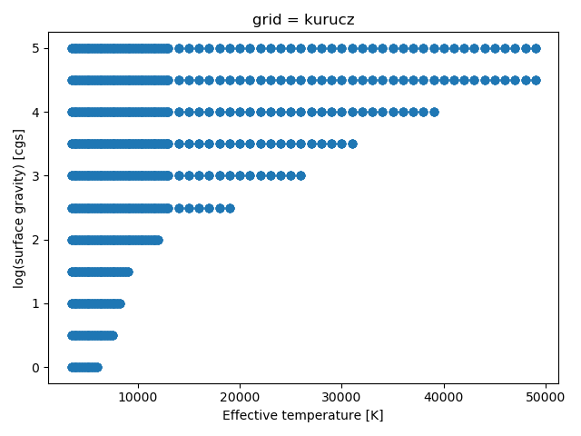
Kurucz
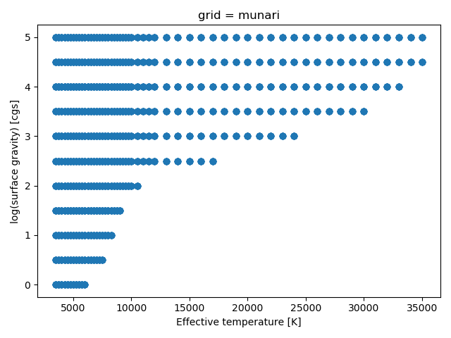
Munari
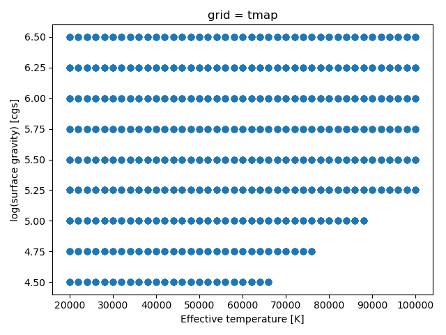
TMAP
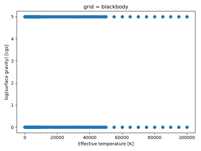
Black body
A black body obviously doesn’t have a surface gravity, but due to the way that the code is build, it is easier to create a pre integrated grid of black body model atmospheres at different temperatures and 2 surface gravities then to change the code and implement the black body analytically.
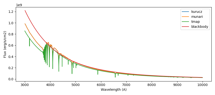
Model comparison
Lets compare a spectrum of each of these models at the same effective temperature and surface gravity:
import pylab as pl
import numpy as np
from speedyfit.model import get_table_single

grids = ['kurucz', 'munari', 'tmap', 'blackbody']

pl.figure(figsize=(10,5))

for grid in grids:

    wave, flux = get_table_single(teff=20000, logg=5.0, ebv=0.0, grid=grid)
    s = np.where((wave > 3000) & (wave<10000))
    pl.plot(wave[s], flux[s], label=grid)

pl.xlabel('Wavelength (A)')
pl.ylabel('Flux (erg/s/cm2)')
pl.legend(loc='best')
pl.tight_layout()
pl.show()
Adding model grids
You can add your own model atmosphere grids to speedyfit. For this you need a fits file containing the model atmospheres, and a separate file containing the models integrated over the pass bands that you want to use. This grid also needs have the reddening pre calculated for the range you want to include in the fit.
The file name for the non integrated grid is not important. The filename of the integrated grid has to follow: <gridfilename>_lawfitzpatrick2004_Rv3.10.fits
Then add the grid to the file ‘grid_description.yaml’ located in the same folder as the model grids: ‘$SPEEDYFIT_MODELS’
The new grid should then show up when calling:
speedyfit checkgrids